1. Introduction¶

On second thought, let’s not go to Camelot. ’Tis a silly place.

—King Arthur, Monty Python and the Holy Grail

1.1. Why programming?¶

When I suggest to fellow linguists that they might want to take up programming as a way to supercharge their abilities to confront and extract meaning from language data, I get a variety of responses. Among the negative ones, two tend to dominate: a fear that it might be too late to start anyway, and a dismissive attitude in the vein of “why should I even care”.

Let’s examine these concerns in turn. Regarding the first one, it’s never too late, trust me. I myself started programming at uni, and not even in my first year. Back then, I thought I was interested in literary studies, and it took me a while to realize that my interests lay elsewhere. Programming is perhaps the easiest skill to acquire from the comfort of your own home, without the need for formal training (though of course interacting with a live teacher can help jumpstart your learning). There’s a wealth of resources available via the internet, this book being one example, and all you need to take full advantage of them is a computer and an internet connection.

Much like any other learning experience, it’s also a journey that never really ends. There’s always room for improvement and for learning more, so you might as well start now and get on with it. For my part, it’s been almost ten years since I set out, and while I consider myself a fairly proficient programmer by this point, I learn new stuff all the time. If you’re anything like me, that sense of curiosity that got you into linguistics, and perhaps even an academic career, is likely to be rewarded by pursuing programming as well.

I would argue that this sense of curiosity is also what should prevent you from having that second kneejerk negative response, “why should I even care”. For my part, I can tell you that programming is very likely the most useful skill I acquired since learning to read. It really expanded the range of what I’m able to achieve not just in linguistics, but in everyday life as well. Our society increasingly relies on software to go about its daily business, and being able to program puts me in much better control of the tools I must willy-nilly use to be a part of it.

One concrete example: have you ever had a month to provide feedback on a Microsoft Word document, only to find yourself pulling an all-nighter just before the deadline because there just wasn’t time earlier, and feeling ashamed of the trail of 3AM timestamps you’re leaving behind? Word offers the nuclear option of removing all metadata in tracked changes and comments across the board, but that includes author names, which is very conspicuous and feels like an even more flagrant admission of guilt, plus if there are multiple authors, you might need to keep them anyway. Luckily, it turns out you can tease the document apart using a Python script and selectively target those pesky timestamps associated with your username. (If this doesn’t sound familiar at all, then congratulations, you don’t have OCD!)

But admittedly, these are just words, to see for yourself, you’re going to have to get your hands dirty and spend some time learning what programming feels like, and what it empowers you to do, what new, unsuspected perspectives it opens. This book is an attempt to help you get started on that path. And if it doesn’t strike a chord with you, it might at least point you to other related resources, some of which will hopefully be a better fit.

If on the other hand, it turns out this book is a good fit for you, then great! And if you end up on the fence, then please consider helping us improve it for future readers like you. The source code of this book lives in a GitHub repository. Please open issues with requests for clarification, tips for improvement, or even just typos!

1.2. Target audience¶

This book is intended as an introduction to programming using the Python programming language. No previous programming experience is required, though a basic amount of technical sophistication is needed; you will hopefully acquire a lot more by the time you’re done reading it.

If you’ve programmed before, but not in Python, or even in Python, but not with a focus on language data, you might still glean useful information from this book, though the pace might feel sluggish at times. And even if you feel at home in both these areas, there might be tricks or gotchas addressed herein that will help you further refine your skills, though of course your mileage may vary.

Finally, if you’ve never programmed, have no background in linguistics and are not particularly computer-literate, reading this book might prove somewhat challenging, though not impossible with the right amount of dedication. If you make it through, or at least part-way, your feedback on how to make the parts you struggled with more accessible would be absolutely invaluable!

1.3. Python gives you wings!¶

So what is this Python business all about? I’ve said before that learning programming was to me the most transformative new skill since learning to read, but it can also prove an uphill struggle. Python is a good entrypoint because it strikes a good balance between simplicity and flexibility, making the learning experience fun and rewarding and just enough challenging. The comic below might poke fun at this claim to get overzealous Python advocates off their soapbox, but by the same token, it shows that Python indeed has this sort of general reputation, otherwise the joke wouldn’t work.

Credit: Randall Munroe, XKCD, https://xkcd.com/353/

Jokes aside though (which is sort of hard to do in a language named after Monty Python’s Flying Circus), the key reason why Python exhibits these desirable properties is that it was designed with teachability to curious amateurs as a primary goal, and it has stayed an important concern during the thirty odd years that Python has evolved and matured since its first public release in 1990. The result is an approachable programming language which emphasizes readable and easily understandable code – properties which are crucial for beginners, but which also appeal to many seasoned programmers. After all, the computer doesn’t care, so we might as well make the language as easy as possible for humans to wrap their head around – is the general idea.

I don’t know how well people know ABC’s influence on Python. […] ABC’s design had a very clear, sharp focus. ABC was intended to be a programming language that could be taught to intelligent computer users who were not computer programmers or software developers in any sense.

—Guido van Rossum, creator of Python, in The Making of Python

Python was also designed as a general purpose language, i.e. it is intended to enable its users to build all kinds of programs in a variety of different domains (though as every programming language, it particularly shines in some and is less well-suited for others). A possible disadvantage of this inclusive approach is that it may be a bit harder to find one’s way around the ecosystem of tools and libraries for a particular purpose (e.g. statistics or data science), but it pays off in that you’re not limited by the one intended use, which is a good thing whenever you embark on a bigger project. And Python encourages you to do that, making it relatively easy to split your code into reusable modules and manage the complexity inherent in that.

Contrast this with another high-level programming language that non-programmers often tend to run into – as a linguist, you might be familiar with R. R is very specifically focused on data analysis, the use case it optimizes for is calling existing statistical functions in an interactive session, and for that, it works admirably well. For anything else though, it can get really ugly. Since “regular” users are mostly meant to consume functions rather than write their own, there is a big gap between the elegant way in which these functions are called, and the messy code with which they’re implemented. To be clear, I don’t mean to say that the code is messy because the people who wrote it are bad programmers; it’s messy because R deliberately made some tradeoffs which make it a complicated language to write larger, reusable pieces of code in, while at the same time making these functions somewhat easier to use.

As a consequence, with R, beginners tend to run up against a wall when trying to use it for anything that’s not easily achieved by an existing library, and though it deserves an honorable mention for having a lot of libraries with useful functionality, some of them very well-designed (I’m looking at you, tidyverse), it’s one of the laws of programming that there will always be at least this one thing in your project that there is no existing library for (or maybe there is, but you can’t seem to find it). Not to mention that if you ever get interested in other areas of programming, R’s laser-sharp focus on data analysis can become a drawback, as it makes R programming skills less transferrable.

This is not to say that Python is a panacea to all, or that it doesn’t have drawbacks of its own. It definitely does. My point is simply that it has a much more consistent and gradual learning curve, which makes it less likely you’ll quit in frustration, and helps you graduate from beginner to intermediate to advanced over time. Perhaps you like R – and that’s totally fine – but you never got over that hump which separates people who use R packages from people who write them. Learning Python might actually be a good way to get there, by improving your general programming skills to a point where you’ll feel confident to tackle that uglier side of R.

Python’s philosophy can be summed up by the guiding principles contained in The Zen of Python, which you can print out in a Python session by importing the this module. Especially the first four entries are key to the argument that I’m trying to make here:

import this

The Zen of Python, by Tim Peters

Beautiful is better than ugly.
Explicit is better than implicit.
Simple is better than complex.
Complex is better than complicated.
Flat is better than nested.
Sparse is better than dense.
Readability counts.
Special cases aren't special enough to break the rules.
Although practicality beats purity.
Errors should never pass silently.
Unless explicitly silenced.
In the face of ambiguity, refuse the temptation to guess.
There should be one-- and preferably only one --obvious way to do it.
Although that way may not be obvious at first unless you're Dutch.
Now is better than never.
Although never is often better than *right* now.
If the implementation is hard to explain, it's a bad idea.
If the implementation is easy to explain, it may be a good idea.
Namespaces are one honking great idea -- let's do more of those!

1.4. How to use this book¶

This book actually consists of a series of Jupyter notebooks, which is a file format, recognizable by its .ipynb extension, which intermixes expository prose with programming code. It can be opened using the JupyterLab application, which runs in your browser. In the notebooks, code is stored inside code cells which can be modified and run at will, which encourages interactive exploration and makes learning easier. This is what a code cell looks like:

1 + 1

You can see the code cell’s output right below it – in this case, it’s a plain old 2.

If you can, it’s a great idea to follow along in JupyterLab, running the code in each chapter of the book yourself and tinkering with it. There are several options for that. The easiest one is to use either the Binder or JupyterHub buttons under the icon at the top of the page, which will take care of everything for you and open an interactive version of this text in your browser, without you needing to install anything on your computer.

Note that the second button requires that you have an account at https://jupyter.korpus.cz (attendees of the V4Py summer school do). The notebook corresponding to the chapter you’re reading should automatically open; if it doesn’t, try reloading the page, or as a last resort, navigating to the v4py.github.io folder and opening the appropriate notebook manually.

If you want to install Python on your own computer and run JupyterLab locally, I would suggest using the Anaconda Distribution, which installs Python alongside many popular additional packages and libraries for data analysis. In that case, you’ll be opening JupyterLab via the Anaconda Navigator, and you’ll need to download the notebooks manually (after unzipping, the notebooks are in the content/ subdirectory). If you don’t mind downloading the notebooks individually, you can also use the download button at the top of the page, but that won’t get you any of the additional files that some of the notebooks rely on.

If you want to learn more about using notebooks, here’s a gallery of interesting notebooks to help you get acquainted with the format, including some introductory tutorials on how to use it right. The JupyterLab notebook user interface is described in more detail in their docs. Finally, some usage tips which I personally find useful can be found in the this blog post.

1.5. Diving right in: a frequency analysis of this text¶

To get our feet wet, let’s do a quick frequency analysis of the text you’re currently reading. If you’ve never programmed before, don’t worry if parts (or all) of the code below seems a little mysterious! We’ll cover all of that in much more detail in the following chapters. However, before we dive into the particulars, I think it’s a good idea to get acquainted with what actual useful Python code looks like, so that we have a general picture of where we’re headed. Without a global perspective and a clear goal in our heads, it’s easy to get discouraged by the many seemingly unconnected details that await us along the way.

So take a while to look at each code chunk below, try and figure out what its purpose might be and how it achieves it, try and discover repeating patterns in Python’s syntax and their meaning. Read the commentary and let the programming vocabulary soak into your brain. It’s alright to be confused, it’s OK not to understand precisely what each and every word means. The goal at this point is to get familiar with how Python code looks and how the terminology sounds, even if you don’t fully understand what’s happening yet.

We start by importing HTMLSession from the requests_html library, which contains functionality related to fetching HTML pages from the web. We create a fresh HTMLSession object and store it in the session variable. Think of it as a simple web browser inside Python.

from requests_html import HTMLSession

session = HTMLSession()

We can fetch the page you’re currently reading by calling the get() method of the session object and passing it the link to this website as an argument. We get back an HTTP response.

link = "https://v4py.github.io/intro.html"
response = session.get(link)

Inspecting the response variable, we see <Response [200]>. 200 is the HTTP status code which indicates that all went well with our request and we received a sucessful response.

response

<Response [200]>

If we don’t know or remember which HTTP status code is which, we can check that everything is fine by inspecting the .ok attribute on the response object.

response.ok

True

The contents of the web page are stored in the .html attribute of the response object.

response.html

<HTML url='https://v4py.github.io/intro.html'>

That attribute is itself an object with attributes and methods of its own, which allow us to inspect it and manipulate it. For instance, it has in turn its own .html attribute, which contains the raw HTML code underlying the web page you’re reading, stored as a string of characters. We can take a look at a slice of the first 50 characters of the string using the [:50] syntax, just to make sure we downloaded the right document. If you’re running this notebook inside JupyterLab, you can delete the square brackets and inspect the full HTML; I’ve not done that here to save some space.

response.html.html[:50]

'\n<!DOCTYPE html>\n\n<html>\n  <head>\n    <meta charse'

Uh-oh, I don’t remember reading anything about any doctypes at the beginning of this text. What’s this all about? Well this is all part of the HTML language, which tells your browser how to display this web page. Trouble is, from our point of view as linguists, this is just junk that we need to get rid of. One thing we could try is the .text attribute, which extracts only the text parts of a web page.

# the first 50 characters
response.html.text[:50]

'1. Introduction — An Introduction to Python for Li'

# the last 50 characters
response.html.text[-50:]

'le under the terms of the CC BY-NC-SA 4.0 license.'

That looks promising, although this still includes header and footer text which we might want to exclude from our analysis if we’re being pedantic. Furthermore, JavaScript programs (which add interactivity to the page; surrounded by <script/> tags) or CSS styles (which define the layout and other aesthetic aspects of the page; surrounded by <style/> tags) might be hiding in the middle of all this. These elements are invisible when you read the rendered page in a browser, but unfortunately, they count as “text”.

More broadly, some pages simply might not be so well-behaved and yield such good results out-of-the-box. So let’s learn a technique to zero in on what you want in a sea of HTML.

We first need to figure out which parts of the HTML enclose the content we’re interested in. For that, we’ll use our browser’s inspector tools. If you right click anywhere on this page, you should get a menu where one of the items says something like Inspect or Inspect Element. Click on that and a pane will open beside the page which lets you peek under the hood of this page. If you right click on this paragraph specifically and select Inspect Element, the inspector will focus on where in the HTML hierarchy this particular paragraph is placed.

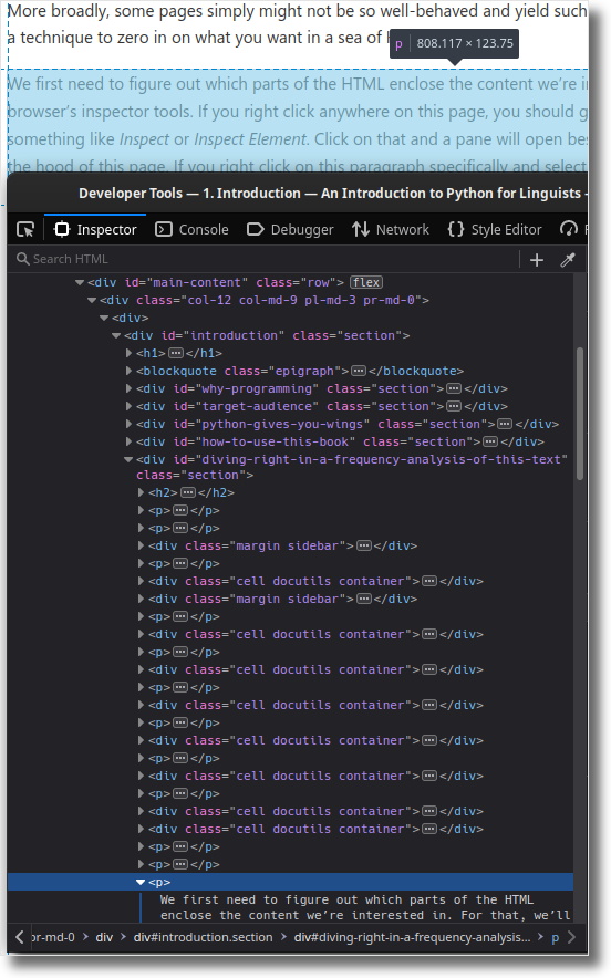
We can see that this paragraph is ultimately contained within a <div/> HTML element which has an ID of main-content. This sounds promising – hopefully, all of the main, interesting content on the page should be placed under this div somewhere, otherwise the ID is a real misnomer. So let’s go on a limb here and retrieve that div using the .find() method. This method uses CSS selectors to slice and dice the page; all we need to know right now is that the syntax to find an HTML element by its ID is to prefix the ID with a hash symbol (also called pound sign or octothorpe), so #main-content in our case. We get back a list of divs; the clean=True keyword argument makes sure that we throw away those pesky invisible <script/> and <style/> tags, if any.

divs = response.html.find("#main-content", clean=True)
divs

[<Element 'div' id='main-content' class=('row',)>]

Apart from id attributes, another common way of selecting HTML elements is via class attributes. Each element should have only one, unique id, but it can have multiple classes and share them with other elements. E.g. on the page you’re reading, all of the cells with Python code live inside divs with a class of cell_input (see for yourself with Inspect Element). The resulting lists can thus easily have more than one element. Try it out! Class selectors start with . instead of #. And here’s how you can join a list of divs into one big string using \newlines: "\n".join(div.text for div in divs).

The list has a single div element, which makes sense – IDs should be unique, so the entire document has just one element which matches the selector #main-content. We can again use the [...] syntax to reach into the list, but this time, we put a single number between the square brackets, because we want to access a single element, not a slice. Additionally, lists in Python are numbered starting from 0, so the way to refer to the first and only item in the list is as divs[0]. We can then retrieve the text inside the div as one long string via its .text attribute, as previously.

string = divs[0].text
string[:30]

'1. Introduction¶\nOn second tho'

string = divs[0].text
string[-30:]

't\n2. A tour of Python and NLTK'

This is starting to look good! Just to see how much stuff we’ve gotten rid of, we can compare the number of characters using the len() function.

len(response.html.full_text), len(response.html.text), len(string)

(33870, 32843, 31345)

(Hmpf. That’s not a whole lot – in this case, we’re probably just being pedantic. But like I said, in general, the results out-of-the-box can vary, or you might want to focus on just part of the content, so this technique is still worth knowing about.)

Now in order to do a frequency analysis, we need to split that text into words or tokens, which is a technical term used when we want to avoid the kind of philosophical hairsplitting that linguists sometimes engage in with respect to what is or is not a word. Referring to words as ‘tokens’ is basically a way of saying, “I don’t want to pick a fight about the precise meaning of ‘word’ right now, I made a pragmatic decision to split the text into pieces which broadly make sense, but of course reasonable people might disagree on the details.” It also allows us to be precise that we are referring to specific instances of words. The word ‘word’ is ambiguous, a sentence like “I know I screwed up.” can be described as containing either 5 (total running) words or 4 (different) words. If we want to avoid confusion, we can say instead that it consists of 5 tokens and 4 types.

Word-splitting or tokenization is a trickier problem than it might seem at first glance, because punctuation keeps getting in the way. So let’s not do it manually ourselves, let’s use instead the word_tokenize() function in the nltk library, which hopefully covers some of the edge cases we wouldn’t think of right off the bat if we were to implement it ourselves off the top of our head. This function returns a list of strings, and again we can do a sanity check by inspecting a slice of it.

import nltk

tokenized = nltk.word_tokenize(string.lower())
tokenized[100:115]

['of',
 '“',
 'why',
 'should',
 'i',
 'even',
 'care',
 '”',
 '.',
 'let',
 '’',
 's',
 'examine',
 'these',
 'concerns']

Looks fine. Notice that before tokenizing the string, we converted in to lowercase using the .lower() method. This is because in our frequency analysis, we probably don’t want to make a distinction between e.g. token and Token. They refer to the same thing, so they should be counted together, but the computer doesn’t know that, as far as it’s concerned, token is as different from Token as it is from grapefruit, so it’s our job to make them exactly the same by lowercasing everything beforehand. We can measure the length of the list and thus get the number of tokens using the len() function.

len(tokenized)

That’s quite a lot, thanks for reading so far!

But hang on, that count is likely to be somewhat inflated. First of all, a lot of the tokens in the tokenized list are junk, at least linguistically speaking, they are special characters related to the notebook format.

tokenized[:15]

['1.',
 'introduction¶',
 'on',
 'second',
 'thought',
 ',',
 'let',
 '’',
 's',
 'not',
 'go',
 'to',
 'camelot',
 '.',
 '’']

Second of all, it doesn’t take a linguist to realize that the most common words in an English text will be words like a or the. We probably don’t want to include those in our frequency analysis, since they’re not very interesting, they don’t tell us a lot. Luckily, nltk has a list of these uninteresting stopwords for English which we can load and store in a set, so that we can quickly check if a given token is a stopword or not. The stopwords are stored in their lowercase form, so it comes in handy that we already lowercased our input string prior to tokenizing it.

from nltk.corpus import stopwords

stop_list = stopwords.words("english")
stop_set = set(stop_list)
stop_list[:15]

['i',
 'me',
 'my',
 'myself',
 'we',
 'our',
 'ours',
 'ourselves',
 'you',
 "you're",
 "you've",
 "you'll",
 "you'd",
 'your',
 'yours']

We can now get rid of any unwanted tokens. The following code snippet is a bit more complicated than the previous ones, it involves some non-linear control flow, which is a fancy way of saying the code doesn’t just linearly execute from top to bottom, but it can run around in circles for a while (the for statement) or potentially skip some parts depending on whether a condition evaluates to true or false (the if statement).

# create a new empty
cleaned = []
# iterate over all the tokens in the tokenized list
for token in tokenized:
    # check if current token is "interesting"
    if token.isalpha() and token not in stop_set:
        # if so, append it to the cleaned list
        cleaned.append(token)
len(cleaned)

cleaned is a lot shorter than tokenized, so it looks like it worked!‡ Note how Python uses indentation to encode the hierarchy of statements in the code: everything which is indented under the for-loop header on the second line is part of the for-loop body and gets executed for each token in the tokenized list. Similarly, everything indented under the if header only gets executed if the conditional expression is satisfied. By dedenting, we escape the tyranny of those fors and ifs, so that the last line gets executed only once, after the for-loop has completed.

Notice also that with suitably chosen variable names, Python code can read almost like English. Readability is one of Python’s main strengths, though it can sometimes be a pitfall for beginners – when they’re not sure how to do something in Python, they try to write it in an English-like way and hope for the best, but this approach can yield valid Python code which however does something different than the plain English interpretation would suggest.

We are now finally in a position to create a frequency distribution, using the nltk.FreqDist class. It’s easy, we just pass it our list of clean tokens.

freq_dist = nltk.FreqDist(cleaned)
freq_dist

FreqDist({'python': 49, 'code': 27, 'programming': 24, 'get': 22, 'one': 22, 'might': 20, 'like': 19, 'page': 17, 'way': 16, 'using': 16, ...})

We can access individual values inside the frequency distribution by requesting them using the corresponding key.

freq_dist["python"]

We can also list the top \(n\) items using the .most_common() method.

freq_dist.most_common(10)

[('python', 49),
 ('code', 27),
 ('programming', 24),
 ('get', 22),
 ('one', 22),
 ('might', 20),
 ('like', 19),
 ('page', 17),
 ('way', 16),
 ('using', 16)]

Based on the most frequent lexical items, it looks like this is a text about Python programming and language data! That checks out.

Finally, we can visualize this result using a wordcloud, to get a quick and intuitive overview of these important words.

from corpy.vis import wordcloud

wordcloud(freq_dist, size=(800, 400), rounded=True)

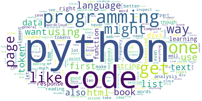
<wordcloud.wordcloud.WordCloud at 0x7fd194daa520>

Whew! That was actually a lot of work. Now that we’ve figured out how to do this, we could package all of these steps into a reusable recipe, so that we don’t have to re-cobble all of this together if we want to run a same analysis on a different chapter. We can do so by writing a function. Again, as with for-loops and if statements, everything that’s indented under the function header starting with def is part of the function body, and will be run step by step each time the function is called.

def chapter_wordcloud(link, size=(800, 400), rounded=True):
    session = HTMLSession()
    response = session.get(link)
    divs = response.html.find("#main-content", clean=True)
    # we expect just one div, abort if there are more, otherwise we'd
    # silently ignore some content (it shouldn't happen, but just in
    # case)
    assert len(divs) == 1, "Expected one div with ID main-content, found more!"
    string = divs[0].text
    tokenized = nltk.word_tokenize(string.lower())
    stop_set = set(nltk.corpus.stopwords.words("english"))
    cleaned = []
    for token in tokenized:
        if token.isalpha() and token not in stop_set:
            cleaned.append(token)
    # if we want just the wordcloud, we can also directly create it from
    # a list of tokens, without making an intermediate nltk.FreqDist
    return wordcloud(cleaned, size=size, rounded=rounded)

The return keyword specifies the result that the function spits out at the other end. Once the function reaches a return statement, it stops execution and gives the result back to whoever called the function.

We can now easily create a wordcloud based on the final chapter of this book, for comparison.

chapter_wordcloud("https://v4py.github.io/outro.html")

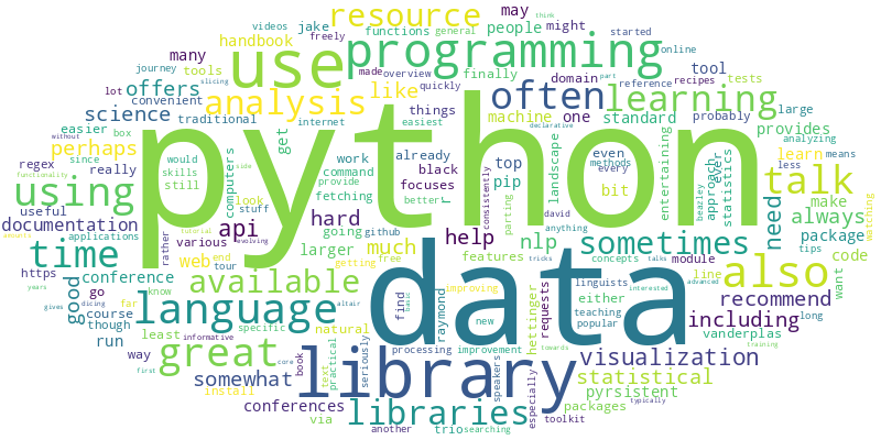
<wordcloud.wordcloud.WordCloud at 0x7fd1963f1100>

Indeed, we can use this function on any chapter in any online book created (much like the present book) with the jupyter-book package, because they all use the same HTML structure. For instance, here’s a wordcloud of the chapter on Regular Expressions from the book Principles and Techniques of Data Science.

chapter_wordcloud("https://www.textbook.ds100.org/ch/13/text_regex.html")

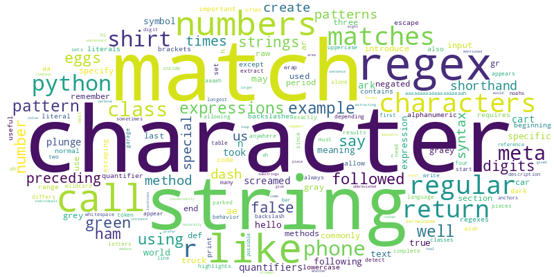
<wordcloud.wordcloud.WordCloud at 0x7fd194af1730>

This is the real power of programming: once you’ve figured out and tweaked a processing and analysis recipe, you can apply it to similar data with lightning speed and each time consistently in exactly the same way.

To wrap up, let me reiterate that I realize this is a lot to take in if this is your first time seeing Python code, and even more so if this is your first time seeing any programming language code whatsoever. Again, it’s totally fine if you don’t understand all the details at this point. I encourage you to revisit this extended worked example once you’re done reading the book, as a way to reflect on what you’ve learned and bring it all together.

An Introduction to Python for Linguists